| Lesson 4 | The EXPLAIN PLAN utility |
| Objective | Run an EXPLAIN PLAN statement. |
Oracle EXPLAIN PLAN Utility, Path Information and Execution Statement
Running an EXPLAIN PLAN is a fairly straightforward process.
The following series of images will demonstrate the process.
- After the PLAN TABLE has been created, we must populate it with access path information by running the SQL statement prefaced with the following:
EXPLAIN PLAN SET STATEMENT_ID = ‘test1’
FOR <<ADD YOUR SQL HERE >>
- Once the access path information has been created, we run the plan.sql script, and analyze the output.
The following series of images will demonstrate the process.
Create Plan Table
1) SQL*Plus Release 3.3.4.0.0 - Production on Mon Oct 18
We create the PLAN TABLE by running the utlxplan.sql script, which always exists in the $ORACLE_HOME/rdbms/admin directory.
SQL > delete from plan_table;
Once the PLAN TABLE has been created, we must populate it with access path information. This is done by running EXPLAIN PLAN SET STATEMENT_ID = 'test1' FOR
set pages 9999;At this point, the SQL optimizer has only been directed to compute the access place and place it in the PLAN TABLE. To view the contents of the PLAN TABLE, we need to execute a snippet of SQL, plan.sql.
SQL>
SQL> @plan
The EXPLAIN PLAN output, if read correctly, reveals vital information. In the case above, two index range scans using the named indexes are run. Next and equi-join (the AND-EQUAL) merges the results of the index range scans. This creates a list of index ROWID's that are passed to a full-table scan of the MON_RTAB_STATS table. Finally, the SORT statement directs Oracle to sort the result set, either in-memory or in the TEMP tablespace.
- We create the PLAN TABLE by running the utlxplan.sql script,
- Once the PLAN TABLE has been created, we must populate it with access path information.
- At this point, the SQL optimizer has only been directed to compute the access place and place it in the PLAN TABLE.
- The EXPLAIN PLAN output, if read correctly, reveals vital information.
All SQL tuning experts must be
Oracle SQL tuning DBAs reveal the explain plans to check many things:
- proficient in reading Oracle execution plans and
- understand the steps within explain plans and
- the sequence in which the steps are executed.
Oracle SQL tuning DBAs reveal the explain plans to check many things:
- Ensure that the tables will be joined in optimal order.
- Determine the most restrictive indexes to fetch the rows.
- Determine the best internal join method to use (e.g. nested loops, hash join).
- Determine that the SQL is executing the steps in the optimal order.
Now that we have a broader understating of how to use the EXPLAIN PLAN, let us try out our new skills by seeing how to detect full-table scans.
Reading Oracle Plan Table
Before moving on to the next lesson, click the Exercise link to try your hand at creating a PLAN table and analyzing an output.
Reading Oracle Plan Table.
Reading Oracle Plan Table.
Oracle Execution Plan
An execution plan shows the detailed steps necessary to execute a SQL statement. These steps are expressed as a set of database operators that consume and produce rows. The order of the operators and their implementations is decided by the query optimizer using a combination of query transformations and physical optimization techniques. While the display is commonly shown in a tabular format, the plan is in fact tree-shaped.
For example, consider the following query based on the SH schema (Sales History):
SELECT prod_category, AVG(amount_sold)
FROM sales s, products p
WHERE p.prod_id = s.prod_id
GROUP BY prod_category;
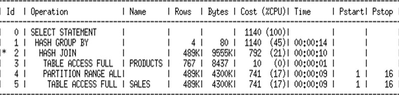
The tabular representation of this query's plan is:
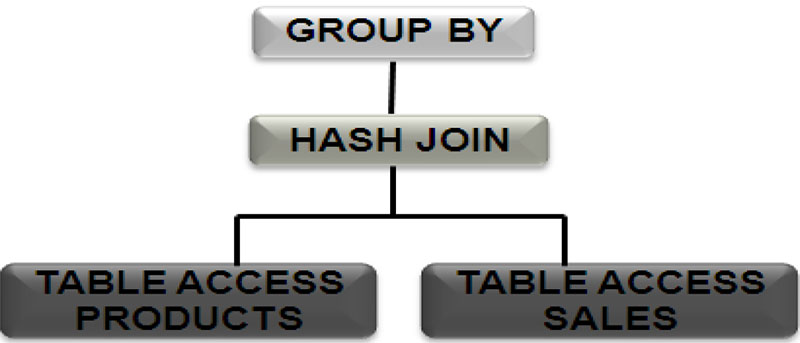
While the tree-shaped representation of the plan is:
Tabular Representation
The tabular representation is a top-down, left-to-right traversal of the execution tree.
When you read a plan tree you should start from the bottom left and work across and then up. In the above example, begin by looking at the leaves of the tree. In this case the leaves of the tree are implemented using a full table scans of the PRODUCTS and the SALES tables. The rows produced by these table scans will be consumed by the join operator. Here the join operator is a hash-join (other alternatives include nested-loop or sort-merge join). Finally the group-by operator implemented here using hash (alternative would be sort) consumes rows produced by the join-operator, and return the final result set to the end user.
This is a cost-based query, since the “cost” hint is used.
We should be suspicious of the TABLE ACCESS FULL statement, since this is very slow. The student should recommend:
This is a cost-based query, since the “cost” hint is used.
We should be suspicious of the TABLE ACCESS FULL statement, since this is very slow. The student should recommend:
- Check for proper index on this table.
- Try re-explaining this query with a “rule” hint.