Lesson 1

Relational databases are the backbone of nearly every application you use today. Whether you are querying a banking system, an e-commerce platform, or a hospital records system, a relational database management system is organizing, protecting, and serving that data behind the scenes. Understanding how relational databases work — and how the software that manages them is architected — is the first step toward writing SQL that is not just functional, but efficient and well-informed.

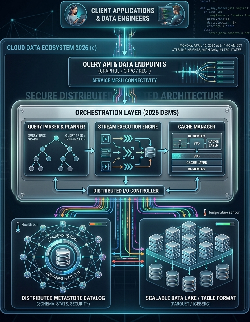
This module introduces relational databases from the ground up. By the time you complete it, you will understand what a normalized database is, why normalization matters for the SQL queries you write, and how modern database management systems have evolved from simple client/server designs into distributed, cloud-native orchestration platforms. The diagram on this page illustrates exactly that evolution — a 2026 cloud data ecosystem showing every architectural layer from the client application down to the physical storage tier.

A relational database organizes data into tables — structured grids of rows and columns — and establishes relationships between those tables using shared values called keys. The word "relational" does not mean that the tables are simply related to one another in a loose sense; it refers specifically to the relational model, a formal mathematical framework introduced by Edgar F. Codd at IBM in 1970. Under the relational model, every table is treated as a mathematical set, and every query operation — selecting rows, joining tables, filtering results — corresponds to a set operation with a precise, provable outcome.

This mathematical grounding is one of the reasons relational databases have remained commercially dominant for more than fifty years. The model is rigorous enough to guarantee consistency and correctness, yet its surface representation — tables, rows, and columns — is familiar to anyone who has ever worked with a spreadsheet or a filing cabinet. That combination of mathematical power and intuitive structure made relational databases accessible to a wide range of professionals, not just computer scientists.

Organizing Data by Common Characteristics

A relational database matches and groups data by using common characteristics found within a dataset. Consider a table of stock transactions. That dataset can be grouped by date range, by price range, by ticker symbol, or by the account that executed the trade. Each grouping reflects a different relational lens on the same underlying data. The schema — the formal definition of tables, columns, data types, and relationships — determines which groupings are possible and how efficiently they can be performed.

When you write a SQL SELECT statement with a WHERE clause or a GROUP BY clause, you are directly exploiting this characteristic-based organization. The database engine evaluates your query against the schema and returns exactly the subset of data that matches your criteria. This is not a coincidence of design — it is the relational model working exactly as Codd intended.

The Mathematical Foundation — Tables as Sets

The mathematics underlying relational databases treats every table as a set of tuples, where each tuple is a row and each attribute in the tuple corresponds to a column. Set theory provides the operations: union combines rows from two compatible tables, intersection returns rows common to both, and difference returns rows in one table but not the other. SQL's JOIN operations are extensions of the Cartesian product — combining every row in one table with every row in another — filtered by a condition that identifies the matching rows.

This set-theoretic foundation has a practical consequence that matters for SQL developers: the order of rows in a table is undefined. A table is a set, and sets have no inherent ordering. When you need results in a specific order, you must explicitly request it with an ORDER BY clause. The database engine is free to return rows in any order that is most efficient for its internal processing — and it will, unless you tell it otherwise.

Why Relational Databases Became Commercially Dominant

During the 1970s and 1980s, several competing data models existed: hierarchical databases organized data as trees, network databases used graph structures, and object databases stored data as programming objects. Each had technical merits. Relational databases won not because they were the most technically sophisticated option, but because they combined three properties that no competing model matched simultaneously: a simple, non-procedural query language (SQL), a mathematically verifiable consistency model, and a schema representation that business users could read and understand without specialized training.

Today, relational database management systems — products like PostgreSQL, MySQL, Oracle Database, Microsoft SQL Server, and IBM Db2 — handle the majority of transactional workloads in enterprise computing. The relational model has also influenced the design of non-relational systems; many NoSQL and NewSQL databases have added SQL-compatible query interfaces precisely because the relational query model is so well understood and so widely taught.

The diagram at the top of this page depicts what a production database environment looks like in 2026. It is worth studying carefully, because it shows the full stack that sits between a developer writing a SQL query and the physical disk where the data is stored. Each layer in the diagram corresponds to a real architectural concern that database designers and data engineers must understand.

Client Applications and Data Engineers

At the top of the diagram are the two primary consumers of a modern database system: client applications and data engineers. Client applications are the software systems that submit queries — web applications, mobile apps, reporting tools, and business intelligence platforms. Data engineers are the professionals who design pipelines, maintain schemas, monitor query performance, and ensure that data flows correctly from source systems into the database and back out to consumers.

The separation of these two roles is significant. In the early years of relational databases, a single database administrator often handled both application-facing queries and backend data management. Modern cloud environments have made the data stack complex enough that these responsibilities are now routinely split across dedicated roles. As a SQL developer, you will interact with both worlds: writing queries that serve application logic, and occasionally participating in the schema and pipeline decisions that data engineers own.

Query API Layer — GraphQL, gRPC, and REST

Between the client and the database engine sits the query API layer. In modern architectures, clients rarely connect directly to a database using a raw SQL connection string. Instead, they interact through an API that translates high-level requests into database operations. The three protocols shown in the diagram — GraphQL, gRPC, and REST — each represent a different approach to this translation.

REST (Representational State Transfer) is the most widely deployed API style, using standard HTTP verbs (GET, POST, PUT, DELETE) to map to database read and write operations. gRPC is a high-performance remote procedure call framework developed by Google, used when low-latency and high-throughput are priorities — common in microservice architectures where services call each other thousands of times per second. GraphQL, developed by Facebook, allows clients to specify exactly which fields they need in a response, reducing over-fetching and giving front-end developers more control over the data they receive.

For SQL developers, the practical implication is that your queries are often not executing in response to a direct database connection. They are being generated or parameterized by an API layer that sits above the DBMS. Understanding this layer helps you reason about where query performance problems originate — whether in the SQL itself, in the API translation layer, or in the network path between them.

Service Mesh Connectivity

The service mesh layer shown in the diagram handles the network-level concerns that arise when dozens or hundreds of microservices need to communicate with database endpoints reliably and securely. A service mesh manages load balancing, traffic routing, mutual TLS encryption, retries, and circuit breaking — all without requiring individual services to implement these concerns themselves. Tools like Istio and Linkerd are widely used service mesh implementations in cloud-native environments.

From a database perspective, the service mesh is the infrastructure that ensures database connections are authenticated, encrypted, and resilient to network failures. It is the reason that modern cloud applications can connect to databases across availability zones and geographic regions without building custom connection-management logic into every service.

The orchestration layer is the core of the 2026 DBMS architecture. It is where the database engine does its actual work: parsing your SQL, planning the most efficient execution strategy, executing the query across potentially distributed data sources, and managing the caches that keep frequently accessed data fast. The orchestration layer contains three major subsystems: the Query Parser and Planner, the Stream Execution Engine, and the Cache Manager.

Query Parser and Query Tree Optimization

When you submit a SQL statement to a database engine, the first thing the engine does is parse it. Parsing converts the raw text of your SQL into a structured internal representation called a query tree — a hierarchical graph where each node represents an operation (scan a table, apply a filter, join two result sets, sort the output). The query tree captures the logical intent of your SQL independently of how the engine will physically execute it.

Once the query tree is built, the query planner takes over. The planner's job is to find the most efficient physical execution strategy for the logical plan. It evaluates options: should this join use a nested loop, a hash join, or a merge join? Should this filter be applied before or after the join? Is there an index that makes this table scan unnecessary? The planner consults statistics about table sizes, column value distributions, and index availability — information stored in the metastore catalog — and produces an optimized execution plan.

This is why understanding database statistics and indexes matters for SQL developers. When you write a WHERE clause that the planner cannot optimize — because the column is unindexed, or because the statistics are stale, or because the predicate uses a function that prevents index use — the planner falls back to a full table scan, and your query becomes slow. The query tree shown in the diagram represents this optimization process visually: a logical graph that gets transformed into an efficient physical plan before a single row is read from disk.

Stream Execution Engine

Modern database engines do not execute queries sequentially, reading one row at a time from start to finish. They use a pipelined, streaming execution model where multiple operations run concurrently and data flows through the pipeline in batches. The Stream Execution Engine shown in the diagram represents this parallel processing architecture.

In a streaming execution model, the table scan, the filter, the join, and the aggregation can all be running simultaneously on different portions of the data. As the scan produces a batch of rows, those rows flow immediately into the filter stage; rows that pass the filter flow into the join stage; joined rows flow into the aggregation. This overlapping execution dramatically reduces total query time compared to a sequential model where each stage must complete before the next begins.

For large datasets — the kind stored in data lakes and distributed storage systems — streaming execution is not optional. It is the only practical way to process hundreds of millions of rows within a time window that users and applications can tolerate. Understanding that your SQL executes in this streaming, pipelined fashion helps explain why certain query patterns (like those that force early materialization of large intermediate result sets) can create unexpected performance bottlenecks.

Cache Manager — In-Memory, SSD, and Cache Layers

The Cache Manager handles one of the most important performance optimizations in any database system: keeping frequently accessed data close to the processor, where it can be retrieved in microseconds rather than the milliseconds required to read from disk. The diagram shows a multi-tier cache hierarchy: an in-memory tier at the top, an SSD cache layer in the middle, and slower persistent storage beneath.

The in-memory tier holds the hottest data — table pages, index entries, and query result fragments that have been accessed recently or are statistically likely to be accessed again. Memory access times are measured in nanoseconds, making the in-memory cache the single most impactful performance layer in the system. The SSD cache layer serves as a high-speed buffer between memory and traditional spinning disk or network-attached storage, offering access times orders of magnitude faster than mechanical disk while providing far more capacity than RAM.

For SQL developers, cache behavior explains why the first execution of a query is often slower than subsequent executions. The first run must read data from disk into the cache; subsequent runs find the same data already resident in memory and complete much faster. This also explains why database performance benchmarks require careful warm-up periods — cold cache performance is not representative of steady-state production performance.

The Distributed I/O Controller is the bridge layer between the orchestration components above and the physical storage systems below. It manages the routing of read and write requests across potentially many storage nodes, handles parallelism at the I/O level, and coordinates consistency across distributed storage backends. In a single-node database, the I/O layer is relatively simple — read this page from disk, write this page to disk. In a distributed system serving petabytes of data across dozens of storage nodes, the I/O controller becomes a sophisticated routing and coordination engine in its own right.

The bidirectional arrows between the Distributed I/O Controller and both the orchestration layer above and the storage layer below — visible in the diagram — reflect the fact that I/O is not a one-way pipeline. Write operations flow downward from the execution engine through the I/O controller to storage; read results flow upward. Cache invalidation signals flow both directions. The I/O controller must coordinate all of this traffic while maintaining consistency guarantees that higher layers depend on.

At the bottom of the architecture sit the two primary storage systems: the Distributed Metastore Catalog and the Scalable Data Lake. These are not interchangeable — they store fundamentally different kinds of information and serve different purposes in the overall system.

Distributed Metastore Catalog (Schema, Stats, Security)

The Distributed Metastore Catalog is the system of record for everything the database engine needs to know about the data — without the data itself. It stores the schema definitions (table names, column names, data types, constraints, relationships), the statistical summaries that the query planner uses for optimization (row counts, column cardinality estimates, histogram data), and the security policies that govern who can access which tables and columns.

The metastore is what the query planner consults when it is deciding how to execute your SQL. When you create a table with CREATE TABLE, the schema is written to the metastore. When the database engine collects statistics with ANALYZE (or its equivalent), those statistics are written to the metastore. When a database administrator grants a user permission to SELECT from a table, that grant is recorded in the metastore. Every decision the query planner makes is informed by the contents of the metastore catalog.

Consensus-Driven Catalog Replication

The diagram shows the metastore catalog as a Consensus-Ring — a distributed architecture where multiple catalog nodes replicate the schema and statistics data among themselves using a consensus protocol. Consensus protocols (like Raft or Paxos) ensure that all nodes in the ring agree on the current state of the catalog before any update is considered committed. This prevents split-brain scenarios where different parts of the system have conflicting views of the schema.

For practical SQL development, the consensus-driven metastore means that schema changes — adding a column, dropping an index, altering a constraint — are atomic and consistent across the entire distributed system. You will not encounter a situation where one query node sees the new column while another still sees the old schema. The consensus protocol guarantees that all nodes see the same schema state simultaneously, which is essential for correctness in a distributed database environment.

Scalable Data Lake and Table Formats — Parquet and Iceberg

The Scalable Data Lake stores the actual data — the rows and columns that your SQL queries retrieve. In modern cloud architectures, data lakes use open table formats rather than proprietary binary formats. The two formats shown in the diagram, Parquet and Apache Iceberg, represent the current state of the art in open, scalable data storage.

Parquet is a columnar storage format, meaning that all values for a given column are stored contiguously on disk rather than row by row. This layout is highly efficient for analytical queries that read a small number of columns from a very large number of rows — the kind of query that drives business intelligence and data analysis workloads. Instead of reading entire rows and discarding most of the columns, the query engine reads only the column files it needs.

Apache Iceberg is a table format layer that sits above Parquet (and other file formats) and adds relational database features to data lake storage: schema evolution, time travel queries, partition pruning, and ACID transaction guarantees. Iceberg is what allows a data lake — which at its core is just a collection of files in object storage — to behave like a proper relational database table with consistent reads, atomic writes, and a queryable history of past states.

Relational database systems were originally developed because of familiarity and simplicity. Because tables are used to communicate ideas in many fields, the terminology of tables, rows, and columns is not intimidating to most users. During the early years of relational databases (1970s), the simplicity and familiarity of relational databases had strong appeal, especially in comparison with the procedural orientation of other data models that existed at the time. Despite the familiarity and simplicity of relational databases, there exists a strong mathematical basis as the foundation of relational databases. The mathematics of relational databases involves conceptualizing tables as sets. The combination of familiarity and simplicity with a mathematical foundation is so powerful that relational database management systems are commercially dominant.

Tables, Rows, and Columns

Every relational database is composed of tables. A table represents a single entity type — customers, orders, products, transactions — and each row in the table represents one instance of that entity. Each column in the table represents one attribute of the entity: a customer's name, an order's date, a product's price. The intersection of a row and a column holds a single value, and that value's type is constrained by the column's data type definition in the schema.

This structure is deliberately simple. A business analyst who has never written a line of SQL can look at a table definition and immediately understand what data it contains. That readability is not accidental — it is a core design principle of the relational model, and it is one of the reasons relational databases have remained the default choice for transactional data management across five decades of computing evolution.

From Monolithic to Client/Server Architecture

The architecture of DBMS packages has evolved considerably since the 1970s. Early systems were monolithic — the entire DBMS software package was one tightly integrated system running on a single machine. All query processing, storage management, and user interaction happened within the same process on the same hardware. These systems were powerful for their time but imposed severe limits on scalability and concurrent access.

The client/server revolution of the 1980s and 1990s broke the monolith apart. Database servers became dedicated machines whose sole responsibility was storing data and processing queries. Client machines connected to those servers over networks, submitting queries and receiving results. This separation allowed many clients to share a single database server, and it allowed the server hardware to be optimized specifically for database workloads — large memory, fast disks, and high-bandwidth network interfaces.

Client Module vs Server Module

In a basic client/server DBMS architecture, the system functionality is distributed between two types of modules:

1. A client module is typically designed to run on a user workstation or personal computer. Application programs and user interfaces that access the database run in the client module. The client module handles user interaction and provides user-friendly interfaces such as forms- or menu-based GUIs (graphical user interfaces). Modern client modules include tools like DBeaver, Beekeeper Studio, and HeidiSQL, as well as the application code in web and mobile applications that submits parameterized queries to the database.
2. A server module handles data storage, access, search, and other backend functions. The server module receives query requests from client modules, executes them against the stored data, and returns result sets. In a distributed cloud architecture, the "server module" is no longer a single process on a single machine — it is the entire orchestration layer shown in the diagram above, spanning query parsing, stream execution, cache management, and distributed storage.

The client/server model established the separation of concerns that all subsequent database architectures have built upon. Whether you are connecting to a local PostgreSQL instance from DBeaver or submitting a query through a GraphQL API to a distributed cloud database, the fundamental division — a client that requests data and a server that stores and retrieves it — remains the organizing principle.

The Cloud Data Ecosystem 2026 diagram includes two monitoring indicators that are easy to overlook but architecturally significant: the health bar associated with the Distributed Metastore Catalog and the temperature sensor associated with the Scalable Data Lake storage array. These represent a category of database system concern that did not exist in early relational database designs: operational observability.

A modern DBMS is not simply a system that stores and retrieves data. It is a continuously monitored operational platform that tracks its own health, performance, and resource utilization in real time. The health bar on the metastore reflects the consensus ring's replication health — are all catalog nodes in agreement? Is any node lagging behind? Are there unresolved conflicts in the schema state? The temperature sensor on the storage array reflects the physical health of the storage hardware — are any drives running hot in ways that predict failure?

For database administrators and data engineers, these observability signals are inputs to automated alerting systems and capacity planning tools. A degraded metastore health score triggers an alert before the degradation causes query failures. An elevated storage temperature triggers a proactive disk replacement before a drive failure causes data loss. Modern DBMS platforms integrate with observability stacks — tools like Prometheus, Grafana, and OpenTelemetry — to expose these signals as metrics that can be dashboarded, alerted on, and analyzed over time.

As a SQL developer, you may not interact directly with these observability systems in your daily work. But understanding that they exist — and that the database platform you are writing queries against is a continuously monitored operational system — gives you important context for interpreting query performance variability, understanding maintenance windows, and communicating with the operations teams who keep the platform running.

This module will now proceed to examine the specific characteristics of relational databases in more detail, beginning with a comparison of relational databases and flat-file storage systems. The architectural foundation covered in this lesson — from the query API layer through the orchestration engine and down to the metastore catalog and data lake — provides the context you need to understand why relational design decisions matter and how they affect the SQL you write.